一、使用numpy实现两层神经网络

需求：一个全连接ReLU神经网络，一个隐藏层，没有bias。用来从x预测y，使用L2 Loss。
两个线性层、一个relu激活函数
hidden隐藏层使用h进行表示
relu激活函数，max(0,h)
输出y_hat

h = w1×X
a = max(0,h)
y_hat = w2×a

Model = Architectures + Parameters
其中Architectures已经确定，是两成神经网络，中间一个relu
要训练Parameters，首先要进行forward pass前向传播，算出预测参数，然后再拿预测的参数与标准的label算一个loss function，拿到loss之后，通过backward pass，求解出梯度Gradients

numpy ndarray是一个普通的n维array。它不知道任何关于深度学习或者梯度(gradient)的知识，也不知道计算图(computation graph)，只是一种用来计算数学运算的数据结构。

64个输入、输入维度1000维、输出维度10维、隐藏层维度100维
N = 64、D_in = 1000、D_out = 10、H = 100

import numpy as np# N is batch size; D_in is input dimension;
# H is hidden dimension; D_out is output dimension.
N, D_in, H, D_out = 64, 1000, 100, 10# Create random input and output data
x = np.random.randn(N, D_in)
y = np.random.randn(N, D_out)# Randomly initialize weights
w1 = np.random.randn(D_in, H)
w2 = np.random.randn(H, D_out)learning_rate = 1e-6
for t in range(500):# Forward pass: compute predicted y# 下三行为模型架构h = x.dot(w1)h_relu = np.maximum(h, 0)y_pred = h_relu.dot(w2)# Compute and print lossloss = np.square(y_pred - y).sum() # (y_pred - y) * (y_pred - y)然后求和，这里使用的Loss是MSE均方误差损失函数print(t, loss)# Backprop to compute gradients of w1 and w2 with respect to loss# loss = (y_pred - y) ** 2grad_y_pred = 2.0 * (y_pred - y)grad_w2 = h_relu.T.dot(grad_y_pred)grad_h_relu = grad_y_pred.dot(w2.T)grad_h = grad_h_relu.copy()grad_h[h < 0] = 0 #这里使用的是relu函数grad_w1 = x.T.dot(grad_h)# Update weightsw1 -= learning_rate * grad_w1w2 -= learning_rate * grad_w2

二、PyTorch实现上述神经网络

需求：使用PyTorch tensors来创建前向神经网络，计算损失，以及反向传播。
一个PyTorch Tensor很像一个numpy的ndarray。但是它和numpy ndarray最大的区别是，PyTorch Tensor可以在CPU或者GPU上运算。如果想要在GPU上运算，就需要把Tensor换成cuda类型。

需要改动的地方：
np.random.randn()改成torch.randn()
x.dot()改成x.mm()
h_relu.dot()改成h.clamp()，clamp相当于一个夹子，上下都可以固定数值
h_relu.dot()改成h_relu.mm()

损失函数：
np.square(y_pred - y).sum()改为(y_pred - y).pow(2).sum().item()
因为pytorch中是tensor，故需要通过item转换成一个值

h_relu.T.dot()改为h_relu.t().mm()
grad_y_pred.dot()改为grad_y_pred.mm()
grad_h_relu.copy()改为grad_h_relu.clone()
x.T.dot()改为x.t().mm()

完整代码如下：

import torchdtype = torch.float
device = torch.device("cpu")
# device = torch.device("cuda:0") # Uncomment this to run on GPU# N is batch size; D_in is input dimension;
# H is hidden dimension; D_out is output dimension.
N, D_in, H, D_out = 64, 1000, 100, 10# Create random input and output data
x = torch.randn(N, D_in, device=device, dtype=dtype)
y = torch.randn(N, D_out, device=device, dtype=dtype)# Randomly initialize weights
w1 = torch.randn(D_in, H, device=device, dtype=dtype)
w2 = torch.randn(H, D_out, device=device, dtype=dtype)learning_rate = 1e-6
for t in range(500):# Forward pass: compute predicted yh = x.mm(w1)h_relu = h.clamp(min=0)y_pred = h_relu.mm(w2)# Compute and print lossloss = (y_pred - y).pow(2).sum().item()print(t, loss)# Backprop to compute gradients of w1 and w2 with respect to lossgrad_y_pred = 2.0 * (y_pred - y)grad_w2 = h_relu.t().mm(grad_y_pred)grad_h_relu = grad_y_pred.mm(w2.t())grad_h = grad_h_relu.clone()grad_h[h < 0] = 0grad_w1 = x.t().mm(grad_h)# Update weights using gradient descentw1 -= learning_rate * grad_w1w2 -= learning_rate * grad_w2

三、PyTorch中的Gradients可以自动求出来

简单的autograd示例

import torch
# Create tensors.
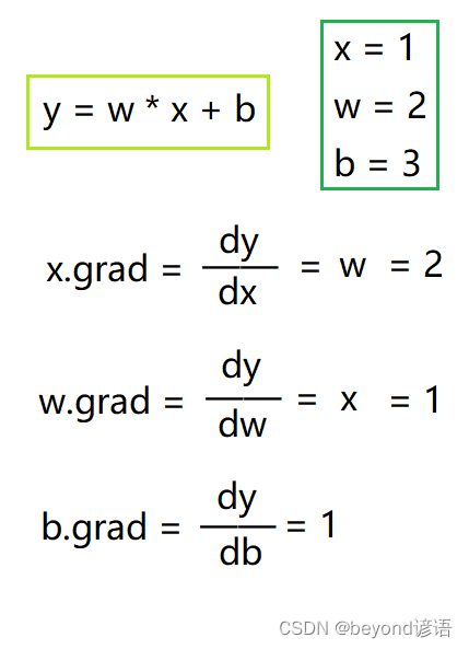
x = torch.tensor(1., requires_grad=True)
w = torch.tensor(2., requires_grad=True)
b = torch.tensor(3., requires_grad=True)# Build a computational graph.
y = w * x + b    # y = 2 * x + 3# Compute gradients.
y.backward()# Print out the gradients.
print(x.grad)    # x.grad = 2 
print(w.grad)    # w.grad = 1 
print(b.grad)    # b.grad = 1 

每次求解的梯度需要重新初始化清零，否则梯度会叠加
w.grad.zero_()
x.grad.zero_()
b.grad.zero_()

代码优化

所以的tensor的运算，在pytorch中都是一个计算图，计算图占用一定的内存空间
故常用with torch.no_grad():

1、PyTorch: Tensor和autograd

PyTorch的一个重要功能就是autograd，也就是说只要定义了forward pass(前向神经网络)，计算了loss之后，PyTorch可以自动求导计算模型所有参数的梯度。

一个PyTorch的Tensor表示计算图中的一个节点。如果x是一个Tensor并且x.requires_grad=True那么x.grad是另一个储存着x当前梯度(相对于一个scalar，常常是loss)的向量。

import torchdtype = torch.float
device = torch.device("cpu")
# device = torch.device("cuda:0") # Uncomment this to run on GPU# N 是 batch size; D_in 是 input dimension;
# H 是 hidden dimension; D_out 是 output dimension.
N, D_in, H, D_out = 64, 1000, 100, 10# 创建随机的Tensor来保存输入和输出
# 设定requires_grad=False表示在反向传播的时候我们不需要计算gradient
x = torch.randn(N, D_in, device=device, dtype=dtype)
y = torch.randn(N, D_out, device=device, dtype=dtype)# 创建随机的Tensor和权重。
# 设置requires_grad=True表示我们希望反向传播的时候计算Tensor的gradient
w1 = torch.randn(D_in, H, device=device, dtype=dtype, requires_grad=True)
w2 = torch.randn(H, D_out, device=device, dtype=dtype, requires_grad=True)learning_rate = 1e-6
for t in range(500):# 前向传播:通过Tensor预测y；这个和普通的神经网络的前向传播没有任何不同，# 但是我们不需要保存网络的中间运算结果，因为我们不需要手动计算反向传播。y_pred = x.mm(w1).clamp(min=0).mm(w2)# 通过前向传播计算loss# loss是一个形状为(1，)的Tensor# loss.item()可以给我们返回一个loss的scalarloss = (y_pred - y).pow(2).sum()print(t, loss.item())# PyTorch给我们提供了autograd的方法做反向传播。如果一个Tensor的requires_grad=True，# backward会自动计算loss相对于每个Tensor的gradient。在backward之后，# w1.grad和w2.grad会包含两个loss相对于两个Tensor的gradient信息。loss.backward()# 我们可以手动做gradient descent(后面我们会介绍自动的方法)。# 用torch.no_grad()包含以下statements，因为w1和w2都是requires_grad=True，# 但是在更新weights之后我们并不需要再做autograd。# 另一种方法是在weight.data和weight.grad.data上做操作，这样就不会对grad产生影响。# tensor.data会我们一个tensor，这个tensor和原来的tensor指向相同的内存空间，# 但是不会记录计算图的历史。with torch.no_grad():w1 -= learning_rate * w1.gradw2 -= learning_rate * w2.grad# Manually zero the gradients after updating weightsw1.grad.zero_()w2.grad.zero_()

2、PyTorch: nn

需求：使用PyTorch中nn这个库来构建网络。 用PyTorch autograd来构建计算图和计算gradients， 然后PyTorch会帮我们自动计算gradient。

nn就是neural network的缩写

通过Sequential将模型中所有层拼接到一起

model = torch.nn.Sequential(torch.nn.Linear(D_in, H, bias=False), # w1*xtorch.nn.ReLU(),torch.nn.Linear(H, D_out),
)

import torch# N is batch size; D_in is input dimension;
# H is hidden dimension; D_out is output dimension.
N, D_in, H, D_out = 64, 1000, 100, 10# Create random Tensors to hold inputs and outputs
x = torch.randn(N, D_in)
y = torch.randn(N, D_out)# Use the nn package to define our model as a sequence of layers. nn.Sequential
# is a Module which contains other Modules, and applies them in sequence to
# produce its output. Each Linear Module computes output from input using a
# linear function, and holds internal Tensors for its weight and bias.
model = torch.nn.Sequential(torch.nn.Linear(D_in, H, bias=False),torch.nn.ReLU(),torch.nn.Linear(H, D_out, bias=False),
)# The nn package also contains definitions of popular loss functions; in this
# case we will use Mean Squared Error (MSE) as our loss function.
loss_fn = torch.nn.MSELoss(reduction='sum')learning_rate = 1e-4
for t in range(500):# Forward pass: compute predicted y by passing x to the model. Module objects# override the __call__ operator so you can call them like functions. When# doing so you pass a Tensor of input data to the Module and it produces# a Tensor of output data.y_pred = model(x) #自动求解model.forward()# Compute and print loss. We pass Tensors containing the predicted and true# values of y, and the loss function returns a Tensor containing the# loss.loss = loss_fn(y_pred, y)print(t, loss.item())# Backward pass: compute gradient of the loss with respect to all the learnable# parameters of the model. Internally, the parameters of each Module are stored# in Tensors with requires_grad=True, so this call will compute gradients for# all learnable parameters in the model.loss.backward()# Update the weights using gradient descent. Each parameter is a Tensor, so# we can access its gradients like we did before.with torch.no_grad():for param in model.parameters(): # param包含tensor和gradparam -= learning_rate * param.grad# Zero the gradients before running the backward pass.model.zero_grad() # 在下一次求导之前，将梯度Gradients清零即可

可以看下模型的架构

model
"""
Sequential((0): Linear(in_features=1000, out_features=100, bias=True)(1): ReLU()(2): Linear(in_features=100, out_features=10, bias=True)
)
"""#看下模型的每一层
model[0] # Linear(in_features=1000, out_features=100, bias=True)
model[1] # ReLU()
model[2] # Linear(in_features=100, out_features=10, bias=True)# 看下模型的权重参数
model[0].weight 
"""
Parameter containing:
tensor([[-0.0159, -0.0271, -0.0346,  ...,  0.0238,  0.0061,  0.0120],[ 0.0290,  0.0258, -0.0142,  ..., -0.0128,  0.0198, -0.0311],[ 0.0209, -0.0169, -0.0307,  ..., -0.0005,  0.0191, -0.0044],...,[ 0.0057, -0.0080,  0.0002,  ...,  0.0317, -0.0025, -0.0027],[-0.0092, -0.0141,  0.0135,  ...,  0.0193,  0.0130, -0.0089],[-0.0163, -0.0309,  0.0054,  ..., -0.0115,  0.0314,  0.0100]],requires_grad=True)
"""model[0].bias # 这里的bias=False，故为没有

3、PyTorch: optim

不再手动更新模型的weights，使用optim这个包来帮助更新参数。
optim这个package提供了各种不同的模型优化方法，包括SGD+momentum, RMSProp, Adam等等。

import torch# N is batch size; D_in is input dimension;
# H is hidden dimension; D_out is output dimension.
N, D_in, H, D_out = 64, 1000, 100, 10# Create random Tensors to hold inputs and outputs
x = torch.randn(N, D_in)
y = torch.randn(N, D_out)# Use the nn package to define our model and loss function.
model = torch.nn.Sequential(torch.nn.Linear(D_in, H, bias=False),torch.nn.ReLU(),torch.nn.Linear(H, D_out, bias=False),
)# 归一化操作
# torch.nn.init.normal_(model[0].weight)
# torch.nn.init.normal_(model[2].weight)loss_fn = torch.nn.MSELoss(reduction='sum')# Use the optim package to define an Optimizer that will update the weights of
# the model for us. Here we will use Adam; the optim package contains many other
# optimization algoriths. The first argument to the Adam constructor tells the
# optimizer which Tensors it should update.
learning_rate = 1e-4
optimizer = torch.optim.Adam(model.parameters(), lr=learning_rate)# 这里也可以使用torch.optim.SGD等多种随机梯度下降方法
for t in range(500):# Forward pass: compute predicted y by passing x to the model.y_pred = model(x)# Compute and print loss.loss = loss_fn(y_pred, y)print(t, loss.item())# Before the backward pass, use the optimizer object to zero all of the# gradients for the variables it will update (which are the learnable# weights of the model). This is because by default, gradients are# accumulated in buffers( i.e, not overwritten) whenever .backward()# is called. Checkout docs of torch.autograd.backward for more details.optimizer.zero_grad()# Backward pass: compute gradient of the loss with respect to model# parametersloss.backward()# Calling the step function on an Optimizer makes an update to its# parametersoptimizer.step()

4、PyTorch: 自定义 nn Modules

定义一个模型，这个模型继承自nn.Module类。如果需要定义一个比Sequential模型更加复杂的模型，就需要定义nn.Module模型。

定义模型，需要初始化__init__()和forward()函数
为了方便，可以把模型定义为一个类TwoLayerNet()

class TwoLayerNet(torch.nn.Module):def __init__(self, D_in, H, D_out): # 定义模型框架"""In the constructor we instantiate two nn.Linear modules and assign them asmember variables."""super(TwoLayerNet, self).__init__()self.linear1 = torch.nn.Linear(D_in, H, bias=False)self.linear2 = torch.nn.Linear(H, D_out, bias=False)def forward(self, x): # 反向传播求梯度"""In the forward function we accept a Tensor of input data and we must returna Tensor of output data. We can use Modules defined in the constructor aswell as arbitrary operators on Tensors."""h_relu = self.linear1(x).clamp(min=0)y_pred = self.linear2(h_relu)return y_pred

import torchclass TwoLayerNet(torch.nn.Module):def __init__(self, D_in, H, D_out):"""In the constructor we instantiate two nn.Linear modules and assign them asmember variables."""super(TwoLayerNet, self).__init__()self.linear1 = torch.nn.Linear(D_in, H, bias=False)self.linear2 = torch.nn.Linear(H, D_out, bias=False)def forward(self, x):"""In the forward function we accept a Tensor of input data and we must returna Tensor of output data. We can use Modules defined in the constructor aswell as arbitrary operators on Tensors."""h_relu = self.linear1(x).clamp(min=0)y_pred = self.linear2(h_relu)return y_pred# N is batch size; D_in is input dimension;
# H is hidden dimension; D_out is output dimension.
N, D_in, H, D_out = 64, 1000, 100, 10# Create random Tensors to hold inputs and outputs
x = torch.randn(N, D_in)
y = torch.randn(N, D_out)# Construct our model by instantiating the class defined above
model = TwoLayerNet(D_in, H, D_out)# Construct our loss function and an Optimizer. The call to model.parameters()
# in the SGD constructor will contain the learnable parameters of the two
# nn.Linear modules which are members of the model.
criterion = torch.nn.MSELoss(reduction='sum')
optimizer = torch.optim.SGD(model.parameters(), lr=1e-4)
for t in range(500):# Forward pass: Compute predicted y by passing x to the modely_pred = model(x)# Compute and print lossloss = criterion(y_pred, y)print(t, loss.item())# Zero gradients, perform a backward pass, and update the weights.optimizer.zero_grad()loss.backward()optimizer.step()

四、总结

由上面的代码思路可以总结得出，PyTorch搭建神经网络模型无非就是以下步骤：
①定义输入和输出的数据
②定义一个模型model
③定义损失函数loss function
④把model交给optimizer去做optim操作
⑤进入一个训练的循环过程，在此过程中，不停的拿训练数据通过模型得出预测的结果，拿到训练预测得到的结果去和真正的结果计算loss，然后计算loss.backward()反向传播，然后调用optimizer.step()去优化参数。

forword pass、计算loss、backward pass、优化模型optimizer.step()

ps：如果你有一个只有一个元素的tensor，使用.item()方法可以把里面的value变成Python数值

五、作业：FizzBuzz

FizzBuzz是一个简单的小游戏。
游戏规则如下：从1开始往上数数，当遇到3的倍数的时候，说fizz，当遇到5的倍数，说buzz，当遇到15的倍数，就说fizzbuzz，其他情况下则正常数数。

我们可以写一个简单的小程序来决定要返回正常数值还是fizz, buzz 或者 fizzbuzz。

思路：首先定义两个函数，函数fizz_buzz_encode()中，负责判断是否是3、5、15的倍数，若是3的倍数，则可以被3整除，余数为0。以此类推，是3的倍数返回1；是5的倍数返回2；是15的倍数返回3；其他的返回0。这里返回的值0，1，2，3就可以将其作为下标索引，列表定义[str(i), "fizz", "buzz", "fizzbuzz"]，若返回0，则索引为0是它本身str(i)；若返回1，则索引为1，是3的倍数，输出fizz；同样的道理，返回2和3也类似。将其整合成一个函数fizz_buzz_decode()。

# One-hot encode the desired outputs: [number, "fizz", "buzz", "fizzbuzz"]
def fizz_buzz_encode(i):if   i % 15 == 0: return 3elif i % 5  == 0: return 2elif i % 3  == 0: return 1else:             return 0def fizz_buzz_decode(i, prediction):return [str(i), "fizz", "buzz", "fizzbuzz"][prediction]print(fizz_buzz_decode(1, fizz_buzz_encode(1)))
print(fizz_buzz_decode(2, fizz_buzz_encode(2)))
print(fizz_buzz_decode(5, fizz_buzz_encode(5)))
print(fizz_buzz_decode(12, fizz_buzz_encode(12)))
print(fizz_buzz_decode(15, fizz_buzz_encode(15)))"""
1
2
buzz
fizz
fizzbuzz"""

根据总结得出的神经网络模型训练步骤进行搭建网络
①定义输入和输出的数据

import numpy as np
import torchNUM_DIGITS = 10# Represent each input by an array of its binary digits.
def binary_encode(i, num_digits):return np.array([i >> d & 1 for d in range(num_digits)])trX = torch.Tensor([binary_encode(i, NUM_DIGITS) for i in range(101, 2 ** NUM_DIGITS)])
trY = torch.LongTensor([fizz_buzz_encode(i) for i in range(101, 2 ** NUM_DIGITS)])

②定义一个模型model
还是用两层线性层和一层relu激活函数模型即可
输入维度10维、隐藏层维度100维、输出维度4维，因为只有0，1，2，3这四个情况

# Define the model
NUM_HIDDEN = 100
model = torch.nn.Sequential(torch.nn.Linear(NUM_DIGITS, NUM_HIDDEN),torch.nn.ReLU(),torch.nn.Linear(NUM_HIDDEN, 4)
)model
"""
Sequential((0): Linear(in_features=10, out_features=100, bias=True)(1): ReLU()(2): Linear(in_features=100, out_features=4, bias=True)
)
"""

③定义损失函数loss function
为了让我们的模型学会FizzBuzz这个游戏，我们需要定义一个损失函数，和一个优化算法。
这个优化算法会不断优化（降低）损失函数，使得模型的在该任务上取得尽可能低的损失值。
损失值低往往表示我们的模型表现好，损失值高表示我们的模型表现差。
由于FizzBuzz游戏本质上是一个分类问题，我们选用Cross Entropyy Loss函数。
优化函数我们选用Stochastic Gradient Descent。

loss_fn = torch.nn.CrossEntropyLoss()
optimizer = torch.optim.SGD(model.parameters(), lr = 0.05)

④把model交给optimizer去做optim操作
⑤进入一个训练的循环过程，在此过程中，不停的拿训练数据通过模型得出预测的结果，拿到训练预测得到的结果去和真正的结果计算loss，然后计算loss.backward()反向传播，然后调用optimizer.step()去优化参数。
这里设置128个输入，开始对模型进行训练，先训练10000轮

# Start training it
BATCH_SIZE = 128
for epoch in range(10000):for start in range(0, len(trX), BATCH_SIZE):end = start + BATCH_SIZEbatchX = trX[start:end]batchY = trY[start:end]y_pred = model(batchX)loss = loss_fn(y_pred, batchY)optimizer.zero_grad()loss.backward()optimizer.step()# Find loss on training dataloss = loss_fn(model(trX), trY).item()print('Epoch:', epoch, 'Loss:', loss)

模型训练好之后，用训练好的模型尝试在1到100这些数字上玩FizzBuzz游戏

# Output now
testX = torch.Tensor([binary_encode(i, NUM_DIGITS) for i in range(1, 101)])
with torch.no_grad():testY = model(testX)
predictions = zip(range(1, 101), list(testY.max(1)[1].data.tolist()))print([fizz_buzz_decode(i, x) for (i, x) in predictions])

print(np.sum(testY.max(1)[1].numpy() == np.array([fizz_buzz_encode(i) for i in range(1,101)])))
testY.max(1)[1].numpy() == np.array([fizz_buzz_encode(i) for i in range(1,101)])